Week 11 - Resilience Patterns: Continued Model Evaluation Patterns. Reproducibility Patterns: Transform and Windowed Inference

Lecture recording here.

Lab recording here.

Introduction

This week we study another resilience pattern: the continued model evaluation pattern. The continued model evaluation pattern can detect when a deployed model is no longer fit-for-purpose by continually monitoring model predictions and evaluating model performance. This is because model performance of deployed models degrades over time either due to data drift, concept drift or other changes to the pipelines which feed data to the model.

We will also look at the transform design pattern and the windowed inference design pattern. The transform reproducibility design pattern ensures that data transformations in processing systems can be consistently reproduced, providing data reliability, traceability, and ease of debugging. The windowed inference design pattern externalizes the model state and invoke the model from a stream analytics pipeline to ensure that features calculated in a dynamic, time-dependent way can be correctly repeated between training and serving.

Videos

Assignment(s)

Assignment 5 - Multimodal Input: An Autonomous Driving System
Assignment 6 - Investigation of Design Patterns for Machine Learning

The Continued Model Evaluation Design Pattern

The Rationale

The rationale for the continued model evaluation pattern is to ensure that machine learning models perform effectively and reliably over time. Its role is to "keep checking if the model is still good." This pattern involves regularly evaluating and monitoring models after they have been deployed in a production environment. The goal is to assess model performance, detect potential issues or drift, and take appropriate actions to maintain or improve model accuracy and reliability.

The Continued Model Evaluation design pattern pattern runs in a continuous loop that

• Collects fresh real-world data from users, sensors, logs, transactions, etc.
• Compare predictions with actual outcomes. It asks the questions did the model guess correctly? How far off was it?
• Measures performance metrics such as accuracy, precision, recall, RMSE,... It also measures drift metrics (data drift, concept drift).
• Trigger actions if performance drops, such as retraining the model, alerting an engineer, switching to a fallback model, and/or start monitoring deeper diagnostics.

The UML

Here is the UML diagram for the continued model evaluation pattern:

  +-------------------+
  |   ModelEvaluator  |
  +-------------------+
  | - model: Model    |
  +-------------------+
  | + evaluate(data)  |
  | + updateModel()   |
  +-------------------+
         /\
         |
         |
         |
         |
         |
  +-------------------+
  |       Model       |
  +-------------------+
  | - parameters      |
  +-------------------+
  | + predict(data)   |
  +-------------------+

1. Model: The Model class represents the predictive model with its parameters and a predict() method that performs the actual prediction based on input data.
2. ModelEvaluator: The ModelEvaluator class is responsible for evaluating the model using the evaluate() method and updating the model using the updateModel() method.

Code Example - Continued Evaluation Pattern

In the provided code, the Model class is implemented with a constructor to initialize model parameters and a predict() method to perform the prediction. The ModelEvaluator class holds an instance of the Model class and provides the evaluate() method to evaluate data using the model. It returns the prediction result based on the model's prediction method. The updateModel() method is used to update the model with new data or retrain the model. In the main() function, you can create a ModelEvaluator object, load the data, evaluate the model using the evaluate() method, and update the model using the updateModel() method. Remember to replace Data with the appropriate data type used in your implementation and adjust the methods and parameters according to your specific requirements.
C++: ContinuedEval.cpp.
C#: ContinuedEval.cs.
Java: ContinuedEval.java.
Python: ContinuedEval.py.

Common Usage

The following are some common usages of the continued model evaluation pattern:

1. Model performance monitoring: Continuously evaluating model performance is crucial to ensure that it meets the desired accuracy and quality standards. Monitoring metrics such as accuracy, precision, recall, F1 score, or area under the curve (AUC) helps identify if the model's performance is degrading or if it is not meeting the desired thresholds. This pattern allows organizations to track the performance of their models and take appropriate actions when performance falls below acceptable levels.
2. Data drift detection: Data used for training models can change over time, leading to data drift. By comparing the distribution of incoming data with the training data, organizations can detect if the model is encountering significantly different data. This helps in identifying potential issues and taking corrective measures, such as retraining the model with updated data or adapting the model to the new data distribution.
3. Concept drift detection: Concept drift refers to the scenario where the relationships between features and target variables change over time. Continuously evaluating models allows organizations to detect concept drift and take necessary actions to address it. This can involve retraining the model with updated data, adjusting model parameters, or even deploying an entirely new model that better captures the changed relationships.
4. Bias and fairness analysis: Evaluating models in production helps uncover biases or fairness issues that may arise in real-world scenarios. By analyzing model predictions across different demographic groups or sensitive attributes, organizations can identify potential biases and take steps to mitigate them. This can involve adjusting training data, feature engineering, or implementing fairness-aware algorithms.
5. Error analysis and improvement: Analyzing the errors made by the model can provide insights into its weaknesses and areas for improvement. By continuously evaluating the model, organizations can identify specific types of errors and patterns, allowing them to refine the model, enhance feature engineering, or apply ensemble techniques to improve overall performance.
6. A/B testing and model version control: The continued evaluation pattern facilitates A/B testing of different model versions. By evaluating multiple models in parallel and comparing their performance, organizations can make data-driven decisions about which model version to deploy in production. It also helps track the performance of different versions over time and provides insights for model version control.
7. Compliance and governance: Continued model evaluation is vital for maintaining compliance with regulatory requirements and governance standards. Organizations can assess whether models are behaving ethically, avoiding discriminatory or biased outcomes. Evaluating models helps ensure transparency, accountability, and adherence to legal and ethical frameworks.

Code Problem - Model Modification

In this example, we have a Data class that represents the input data, containing a vector of features. The Model class represents the model used for prediction, which consists of a vector of weights. The ModelEvaluator class is responsible for evaluating the model using the provided data and updating the model with new weights. In the main() function, we create a ModelEvaluator object with initial weights, load the input data, and evaluate the model using the evaluate() method. The prediction result is then printed to the console. Next, we update the model with new weights using the updateModel() method and evaluate the model again with the updated weights. The updated prediction result is printed to the console.

You can customize the example by modifying the number of features, adding additional evaluation logic, or adjusting the model's prediction mechanism to suit your specific requirements.
Data.h,
Model.h,
Model.cpp,
ModelEvaluator.h,
ModelEvaluator.cpp,
ModelMod.cpp.

Code Problem - Linear Regression Model Modification

This example is similar to the previous. The below code creates a simple linear regression model and continuously evaluates and updates it based on a stream of data. Additionally, multithreading is used to simulate concurrent evaluation and updating.
LinearRegressionModel.h,
DataStreamGenerator.h,
ModelEvaluator.h,
ModelUpdater.h,
LinearRegressionModMain.cpp.

The Transform Design Pattern

The transform design pattern for machine learning focuses on ensuring the reproducibility and consistency of data transformations, which are critical for training, testing, and deploying models. This pattern emphasizes deterministic transformations, version control, and environmental consistency to maintain data integrity and facilitate debugging.

This pattern "Turn your raw data into something the model can understand." Most real-world data is messy, inconsistent, or in the wrong format for an ML model. The Transform pattern describes how to clean, convert, and reshape data before feeding it into a model. This pattern ensures that data goes through a pipeline of transformations so that the final input is model-ready.

The Rationale

The problem is that the inputs to a machine learning model are not the features that the machine learning model uses in its computations. In a text classification model, for example, the inputs are the raw text documents and the features are the numerical embedding representations of this text. When we train a machine learning model, we train it with features that are extracted from the raw inputs. The solution is to explicitly capture the transformations applied to convert the model inputs into features.

The UML

The following is a very basic UML diagram of the transform design pattern.

  +-----------------------------------------------+
  |              Raw Data Source                  |
  |  - Collect data from various sources          |
  +-----------------------------------------------+
                     |
                     v
  +-----------------------------------------------+
  |           Data Ingestion Layer                |
  |  - Ingest and store raw data                  |
  |  - Ensure immutability                        |
  +-----------------------------------------------+
                     |
                     v
  +-----------------------------------------------+
  |       Data Transformation Engine              |
  |  - Apply transformations to data              |
  |  - Ensure transformations are deterministic   |
  |  - Version control for transformation logic   |
  +-----------------------------------------------+
                     |
                     v
  +-----------------------------------------------+
  |           Feature Store Layer                 |
  |  - Store transformed features                 |
  |  - Ensure features are versioned and immutable|
  +-----------------------------------------------+
                     |
                     v
  +-----------------------------------------------+
  |      Machine Learning Model Training          |
  |  - Use versioned features for training        |
  |  - Ensure reproducibility of training process |
  +-----------------------------------------------+
                     |
                     v
  +-----------------------------------------------+
  |       Model Serving and Deployment            |
  |  - Deploy trained models                      |
  |  - Use versioned features for prediction      |
  +-----------------------------------------------+
                     |
                     v
  +-----------------------------------------------+
  |      Monitoring and Feedback Loop             |
  |  - Monitor model performance                  |
  |  - Collect feedback for continuous improvement|
  +-----------------------------------------------+

Code Example - Transform

Below is a simple example of using the transform design pattern for a machine learning workflow. This example demonstrates data normalization, which is a common transformation step. We'll use a basic class to handle the normalization of a dataset.
C++: Transform.cpp.
C#: Transform.cs.
Java: Normalizer.java, Transform.java.
Python: Transform.py.

Common Usage

The transform design pattern is widely used in machine learning for various purposes. Here are some common usages:

1. Data Preprocessing
   Normalization/Standardization: Scaling data to a standard range or normal distribution to improve model performance.
   Encoding Categorical Variables: Converting categorical data into numerical format using techniques like one-hot encoding or label encoding.
   Feature Engineering: Creating new features from existing data to enhance model performance.
   Imputation: Filling in missing values using strategies like mean, median, mode, or predictive models.
2. Data Augmentation
   Image Augmentation: Applying transformations like rotation, scaling, cropping, and flipping to increase the diversity of the training dataset.
   Text Augmentation: Techniques like synonym replacement, random insertion, and back translation to generate more diverse textual data.
3. Dimensionality Reduction
   Principal Component Analysis (PCA): Reducing the dimensionality of the data while preserving as much variance as possible.
   t-Distributed Stochastic Neighbor Embedding (t-SNE): Reducing high-dimensional data into two or three dimensions for visualization purposes.
4. Feature Extraction
   Text Vectorization: Converting text into numerical vectors using methods like TF-IDF, Word2Vec, or BERT embeddings.
   Image Feature Extraction: Using techniques like convolutional neural networks (CNNs) to extract features from images.
5. Data Transformation Pipelines
   Pipeline Construction: Combining multiple preprocessing and transformation steps into a single pipeline to ensure consistency and reproducibility.
   Cross-Validation: Using pipelines to ensure that data transformation steps are correctly applied during cross-validation to prevent data leakage.
6. Model Interpretation
   Shapley Values: Transforming model predictions into contributions of each feature for interpretability.
   LIME (Local Interpretable Model-agnostic Explanations): Generating interpretable explanations for model predictions by transforming data into a locally linear representation.
7. Model Deployment
   Inference Pipeline: Applying the same transformations used during training to new data during inference to maintain consistency.
   Online Feature Transformation: Real-time transformation of data in production systems to ensure incoming data matches the format expected by the model.
8. Time Series Analysis
   Lag Features: Creating lagged versions of time series data for predictive modeling.
   Rolling Window Features: Calculating rolling statistics (e.g., mean, standard deviation) over a fixed window of past data points.
9. Anomaly Detection
   Feature Scaling: Transforming features to detect anomalies more effectively.
   Dimensionality Reduction: Reducing feature space to identify outliers more easily.
10. Synthetic Data Generation
    SMOTE (Synthetic Minority Over-sampling Technique): Generating synthetic samples to balance class distribution in imbalanced datasets.
    GANs (Generative Adversarial Networks): Creating synthetic data that mimics the distribution of the original dataset.

Code Problem - Data Normalization

The following code uses the transform design pattern for data normalization. The loadData function simulates the loading of numerical data: MultiTransform.cpp.
The Normalizer class performs data normalization.
The fit() method calculates the means and standard deviations of the features.
The transform() method normalizes a single feature vector using the stored means and standard deviations.
The fitTransform() method fits the normalizer to the data and then transforms it.

Windowed Inference

The Rationale

The Windowed Inference Pattern is used when the model should not process an entire long sequence at once, but instead breaks the input into fixed-size overlapping or non-overlapping "windows" and runs inference on each window separately. This pattern is especially important for time series, sensor streams, log data, and long text/audio sequences.

"Don't look at all the data at once - look at it in chunks (windows)." Sometimes the data coming into a model is too big, continuous, or arrives in a stream. You cannot process all of it at once. So instead of feeding the entire dataset to the model, you break the data into smaller windows, process each window, and then combine the results.

The Windowed Inference Pattern exists because many ML models cannot process arbitrarily long sequences at once, or because doing so would be computationally expensive, slow, and unnecessary. By splitting the input into fixed-size windows and running inference on each slice, the pattern enables real-time predictions, reduces latency, handles memory limits, preserves temporal relevance, lowers compute costs, and simplifies both training and deployment - especially for streaming, time-series, and log-analysis tasks.

The UML

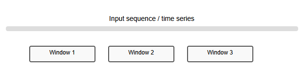
Below is a simplified UML diagram for the Windowed Inference design pattern:

Horizontal bar - "Input sequence / time series". UML equivalent: this is the DataStream or InputSequence object.
It represents a long ordered list of data points, such as timestamps, log entries, sensor readings, or tokens.

Rectangles labeled "Window 1", "Window 2", "Window 3". UML equivalent: each rectangle is an instance of a Window class, representing a slice of the input sequence.
These windows are created by a WindowGenerator or WindowManager component, which takes the long InputSequence, and produces many Window objects (either overlapping or non-overlapping)

Conceptually, each Window is then passed to a Model component, which produces a prediction for that window. The predictions may optionally be sent to an Aggregator that combines the window-level outputs into a final result (for example: maximum, mean, majority vote, or "any window anomalous?").

Below is a more complete UML diagram for the Windowed Inference design pattern:

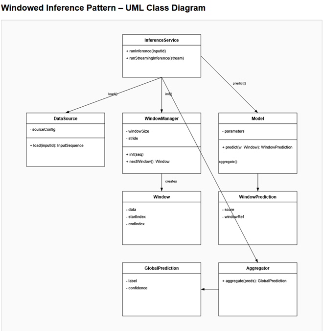
The components are described below:

DataSource. Provides the raw input sequence that will be processed (for example, a list of data points). It passes this sequence to the WindowManager.
WindowManager. Takes the full input sequence and splits it into smaller pieces called Windows (for example, chunks of fixed length). It creates and hands out Window objects one by one.
Window. Represents one slice of the original sequence. It stores the data for that slice and the indices (start and end positions) inside the full sequence. This corresponds to "Window 1", "Window 2", "Window 3" in the diagram.
Model. Takes a single Window as input and produces a prediction for that window (for example, a score or classification).
WindowPrediction. Stores the result of the model's prediction for one Window (for example, a score) and may keep a reference back to that Window.
Aggregator. Combines many WindowPrediction objects into a single overall result (for example, by taking the maximum or average).
InferenceService (or API). Coordinates the whole process: it gets data from DataSource, asks WindowManager for Windows, calls the Model on each Window, sends all WindowPredictions to the Aggregator, and returns the final result to the caller.

Code Example - Windowed Inference

Below is a simple example of using the windowed inference design pattern for machine learning that reflects the idea of splitting sequence into segments, predictions per segment, and aggregation at the end.
C++: WindowedInference.cpp.
C#: WindowedInference.cs.
Java: WindowedInference.java, Python: WindowedInference.py.

Common Usage

1. Financial Trading. Models analyze short windows of recent market data to detect volatility, generate quick trading signals, or estimate short-term risk.
2. Network Security. Systems scan windows of recent network traffic or log entries to spot anomalies such as unusual access patterns or rapid login attempts.
3. Predictive Maintenance. Machines stream sensor data, and models evaluate short time windows to detect signs of wear or early equipment failure.
4. Healthcare Monitoring. Medical devices process windows of ECG, EEG, or wearable data to identify events such as arrhythmias, seizures, or sleep stages.
5. Speech and Voice Assistants. Audio streams are processed in small overlapping windows to detect wake words like “Hey Siri” or “OK Google.”
6. Video Surveillance. Cameras analyze short windows of video frames to detect motion, actions, or unusual activity.

Code Problem - Segmented Prediction

Below is an example that performs segmented prediction using the Windowed Inference pattern. It does not perform real machine learning - it only simulates the flow, demonstrating how windows flow through the pipeline
(DataSource → WindowManager → Model → Aggregator → InferenceService):
DataSource.h, Input provider,
Window.h, Data slice,
WindowManager.h, Window creator,
WindowPrediction.h, Segment result,
Model.h, Predictor,
Aggregator.h, Result combiner,
InferenceService.h, Pipeline controller
SegmentedPred.cpp, Main program.

Additional Exercises (Lab Class)

The below provides scenarios which can be resolved by one (or more) of the machine learning design patterns that we have covered so far. Read the scenario, choose a pattern, and explain your pattern of choice.

1. A hospital wants to build a model that predicts early signs of sepsis.
   In their dataset:
   • Only 2% of patient records indicate early-stage sepsis
   • The remainder are normal cases
   • The model currently predicts “no sepsis” almost all the time, achieving 98% accuracy but missing most true cases

   Question: Which ML design pattern should be applied to most effectively address the extreme class imbalance?
   Correct Answer.

2. A fintech company built an online credit-risk API in Python.
   However:
   • The API must scale horizontally across many containers
   • Each request must be completely independent
   • The system must not rely on previous outputs, cached state, or session memory
   • Containers may start and stop at any time

   Question: Which ML design pattern ensures that each prediction request is fully independent and safely scalable?
   Correct Answer.

3. A manufacturing plant collects temperature and vibration data from machinery at 100 Hz.
   A predictive-maintenance model requires:
   • Fixed-size windows of 5 seconds
   • A stride of 2 seconds (windows overlap)
   • A prediction for each window
   • Results to be aggregated into a fault score

   Question: Which ML design pattern supports chunking the stream into overlapping windows and performing segmented inference?
   Correct Answer.

4. A small startup is building a classifier to categorize customer-support emails.
   Challenges:
   • They have only 400 labelled examples
   • Training from scratch performs poorly
   • A large public dataset exists for general email classification

   Question: Which ML design pattern allows them to leverage an existing pretrained model to improve performance on their smaller dataset?
   Correct Answer.

5. What are the similarities and differences between batch learning and windowed inference?
   Correct Answer.