Week 9 - Patterns that Modify Model Training: Checkpoints, Transfer Learning and Distribution Strategy

Lecture recording here.

Lab recording here.

Introduction

This week we will look at three patterns that modify model training: checkpoints, transfer learning and distribution strategy. The checkpoints pattern stores the full state of the model periodically, so that partially trained models are available and can be used to resume training from an intermediate point, instead of starting from scratch. The transfer learning pattern The transfer learning pattern takes parts of a previously trained model, freezes the weights, and uses these nontrainable layers in a new model that solves a similar problem. This is needed when there is a lack of large datasets that are needed to train complex machine learning models. The distribution strategy pattern carries the training loop out at scale over multiple workers, taking advantage of caching, hardware acceleration, and parallelization.

Video(s)

Assignment(s)

Assignment 4 - Multi-View Machine Learning Predictor
Assignment 5 - Multimodal Input: An Autonomous Driving System

The Checkpoints Design Pattern

The Rationale

The Checkpoints design pattern in machine learning ensures that progress during long or iterative training processes is safely preserved and recoverable. It involves periodically saving the model's state, parameters, and relevant metadata so training can resume from the most recent or best-performing point instead of restarting from scratch after interruptions or failures. This approach improves fault tolerance, enables reproducibility, supports early stopping and model selection, and saves computation time—making it an essential pattern for maintaining reliability and efficiency in real-world ML pipelines.

The UML

1. Trainer. Controls the main training loop. Coordinates learning and delegates persistence to the CheckpointManager so training logic stays clean and restartable.
2. CheckpointManager. Manages creation, loading, and organization of checkpoints. Encapsulates when and where to save or restore progress, applies checkpoint policies, and communicates with storage backends.
3. ModelState. Represents everything needed to resume training. Captures the minimal sufficient state for reproducibility and resumption, serialized and deserialized by the manager.
4. Storage (Interface). Abstracts the persistence mechanism. Allows switching between different storage options without changing higher-level logic.
5. LocalStorage & CloudStorage. Implement the Storage interface. Same interface, different backends - makes it easy to switch from local experiments to distributed training.

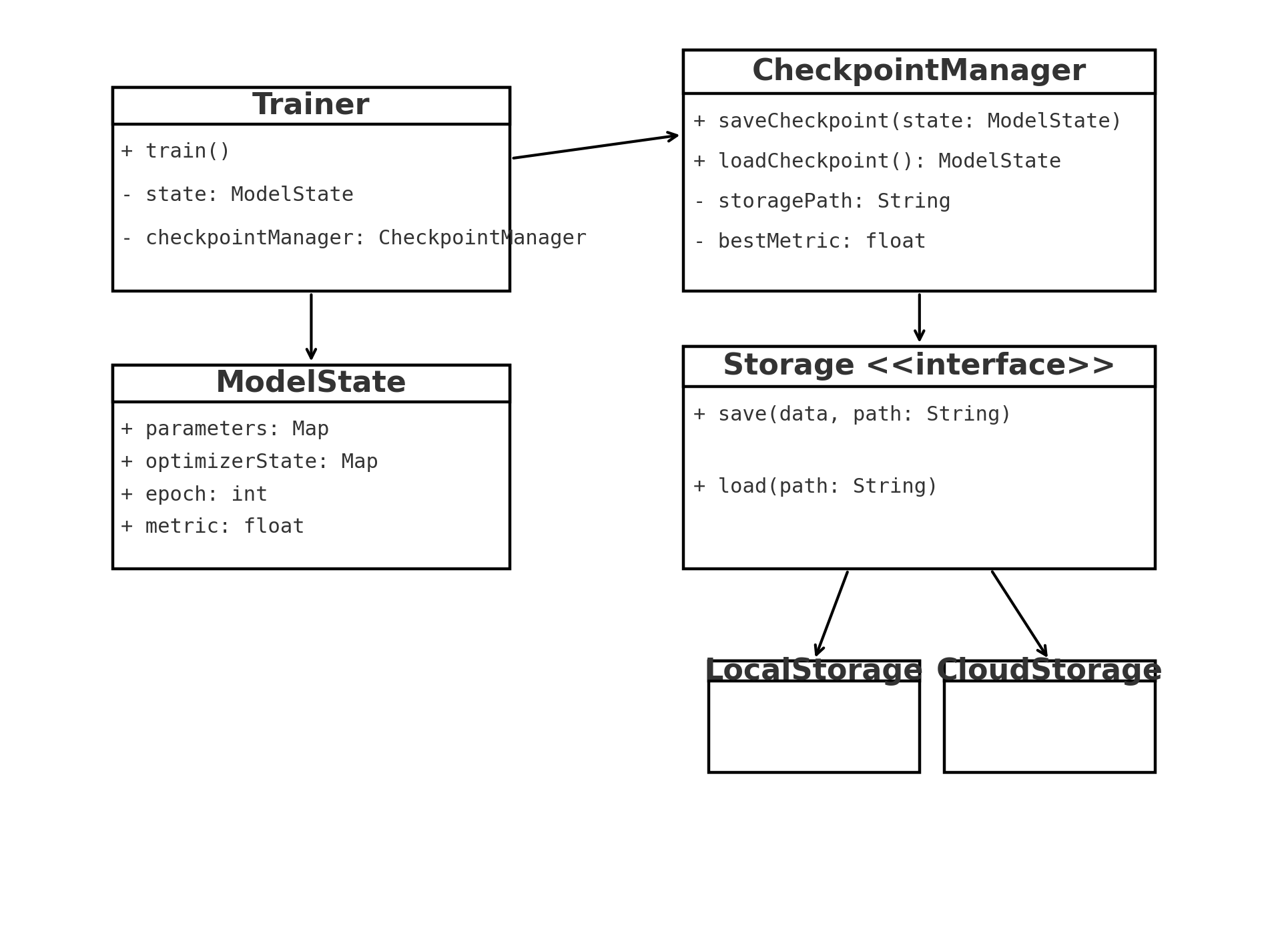
Code Example - Checkpoints

The sample code demonstrates the Checkpoints design pattern, which allows a long-running process (like model training) to save and resume progress safely. It defines a ModelState class to hold the model's state (epoch and performance metric), a Storage interface for saving and loading data, and a LocalStorage class that implements this interface using simple file I/O. The CheckpointManager tracks the best metric achieved so far and saves a checkpoint only when performance improves, while the Trainer class simulates a training loop that updates the model state and delegates checkpointing duties to the manager. Together, these components show how checkpointing separates progress persistence from training logic, improving reliability and fault tolerance in long-running computations.
C++: Checkpoints.cpp,
C#: Checkpoints.cs,
Java: Checkpoints.java,
Python: Checkpoints.py.

Common Usage

the Checkpoints design pattern is a foundational reliability and recovery mechanism across many domains, especially in large-scale computation, machine learning, and data processing. Here are five real-world examples of where it's used in industry:

1. Machine Learning Model Training (TensorFlow, PyTorch). Frameworks like TensorFlow, PyTorch, and Keras use checkpoints to periodically save model weights, optimizer states, and configurations during training. If training is interrupted (e.g., hardware failure, preempted GPU instance), it can resume from the last checkpoint instead of restarting. This is essential for large models like GPT, BERT, or ResNet that can take days or weeks to train.
2. Big Data Processing (Apache Spark, Hadoop). Systems like Apache Spark and Hadoop MapReduce use checkpointing to save intermediate computation states during distributed processing. If a node fails, tasks can resume from the last checkpoint rather than recomputing the entire data flow, ensuring fault tolerance and reducing recomputation time for iterative algorithms like PageRank or K-Means.
3. Streaming Data Pipelines (Apache Flink, Kafka Streams). In real-time data processing systems (e.g., Apache Flink, Kafka Streams), checkpoints are used to maintain exactly-once processing guarantees. The system periodically saves operator states and message offsets so that, in case of failure, it can restore the pipeline to a consistent state without data loss or duplication.
4. High-Performance Computing (HPC) and Simulations. Scientific computing systems (e.g., NASA, CERN, weather forecasting centers) use checkpointing in long-running numerical simulations that can last days on supercomputers. Checkpointing allows restarting simulations from recent states after hardware faults, software crashes, or maintenance downtime, avoiding the loss of expensive compute time.
5. Database and Distributed Systems Recovery. Modern databases (PostgreSQL, MySQL) and distributed systems (Google Spanner, Amazon Aurora) use checkpoints (or similar write-ahead logging concepts) to capture consistent snapshots of in-memory data. After crashes or restarts, the database recovers quickly to a consistent state without replaying all historical operations from scratch.

In short, the Checkpoints pattern is widely used anywhere reliability, fault recovery, or reproducibility are critical — from deep learning and big data to real-time analytics, scientific computing, and distributed storage systems.

Code Problem - Logistic Regression

This C++ program demonstrates an in-memory Checkpoints design pattern applied to logistic regression training. It builds a small machine learning model that performs gradient descent on synthetic data while automatically saving and restoring checkpoints entirely in memory (no files). A CheckpointManager tracks the latest and best model states, managed by an InMemoryStorage class that acts like a volatile database. When the loss diverges (spikes or becomes NaN/∞), the system rolls back to the last best checkpoint, reduces the learning rate, and continues training — ensuring resilience and stability. This example illustrates how checkpointing improves fault tolerance, adaptive learning rate control, and recovery in iterative optimization without relying on external storage.
ModelState.h, the model state structure,
Storage.h, storage interface class,
InMemoryStorage.h, concrete storage,
CheckpointPolicy.h, the checkpoint policy structure,
CheckpointManager.h, the checkpoint manager,
Dataset.h, the dataset structure (complex),
Trainer.h, the trainter structure (complex),
Utilities.h,
Utilities.cpp, some mathematical utilities
LRegress.cpp, the main function.

Memento vs. ML Checkpoints

The Transfer Learning Design Pattern

Transfer learning, used in machine learning, is the reuse of a pre-trained model on a new problem. In transfer learning, a machine exploits the knowledge gained from a previous task to improve generalization about another. For example, in training a classifier to predict whether an image contains food, you could use the knowledge it gained during training to recognize drinks. For more information see What Is Transfer Learning?.

The Rationale

The rationale behind the transfer learning design pattern stems from the observation that deep learning models trained on large-scale datasets can learn generic features that are useful for a wide range of tasks. Transfer learning leverages this idea by reusing pre-trained models as a starting point for new tasks.

The UML

Here is the UML diagram for the transfer learning pattern:

  +---------------------------------+
  |           Pre-trained Model     |
  +---------------------------------+
  |                                 |
  | - Trained on large-scale dataset|
  | - Captures generic features     |
  +---------------------------------+
               ^
               |
  +---------------------------------+
  |        New Task-Specific Model  |
  +---------------------------------+
  |                                 |
  | - Reuses pre-trained model      |
  | - Freezes pre-trained layers    |
  | - Adds new task-specific layers |
  | - Fine-tunes the model          |
  +---------------------------------+

1. Pre-trained Model: This component represents a deep learning model that has been pre-trained on a large-scale dataset (e.g., ImageNet). It captures generic features and knowledge learned from the original task. The pre-trained model serves as a starting point for the transfer learning process.
2. New Task-Specific Model: This component represents the model that is created for the new task using transfer learning. It consists of the pre-trained model as the base, with its layers frozen to preserve the learned features. New task-specific layers are added on top of the pre-trained layers. These additional layers are designed specifically for the new task and are trainable. The model is then fine-tuned on the new task-specific data to adapt the knowledge from the pre-trained layers to the target domain.

Code Example - Transfer Learning

In this code, we have two classes: PretrainedModel and NewTaskModel. The PretrainedModel class represents the pre-trained model, and it has methods to load the pre-trained model weights and extract features using the pre-trained layers. The NewTaskModel class represents the model for the new task. It has methods to add new task-specific layers and perform fine-tuning on the new task-specific data. In the main() function, we create an instance of PretrainedModel and load the pre-trained model weights. Then, we create an instance of NewTaskModel. The transfer learning process involves extracting features from the pre-trained model using pretrainedModel.extractFeatures(), adding task-specific layers using newTaskModel.addTaskSpecificLayers(), and fine-tuning the model on the new task-specific data using newTaskModel.fineTune(). Finally, you can use the trained new task-specific model for inference or any other desired tasks.

Note that this code is a basic representation to illustrate the concept of transfer learning in C++. In practice, you would need to adapt it to the specific deep learning framework or library you are using and incorporate additional functionalities as needed:
C++: TransferLearning.cpp.
C#: TransferLearning.cs.
Java: TransferLearning.java.
Python: TransferLearning.py.

Common Usage

The transfer learning design pattern is commonly used in various scenarios to leverage the knowledge gained from pre-trained models and apply it to new tasks or domains. The following are some common usages of the transfer learning design pattern:

1. Image Classification: Transfer learning is extensively used in image classification tasks. Pre-trained models trained on large-scale datasets, such as ImageNet, are used as a starting point. The learned features from the pre-trained model are extracted and used as input to train a new classifier for a specific set of classes or a different dataset.
2. Object Detection: Transfer learning can be applied to object detection tasks. Pre-trained models, such as Faster R-CNN or SSD, are used as feature extractors. The pre-trained model's convolutional layers are used to extract features from input images, and then additional layers are added to perform object detection on specific classes or datasets.
3. Natural Language Processing (NLP): In NLP tasks, transfer learning can be applied using pre-trained models like BERT or GPT. The pre-trained models are fine-tuned on specific NLP tasks, such as sentiment analysis, named entity recognition, or machine translation. The pre-trained models' language understanding capabilities are leveraged, and additional layers are added for task-specific fine-tuning.
4. Speech Recognition: Transfer learning can be used in speech recognition tasks. Pre-trained models, such as DeepSpeech or Listen, Attend and Spell (LAS), can be used to extract high-level features from audio data. These features are then used to train a new classifier or decoder for specific speech recognition tasks or datasets.
5. Anomaly Detection: Transfer learning can be applied to anomaly detection tasks, where pre-trained models are used to capture the normal behavior of a system or dataset. The pre-trained models' learned representations are used to detect deviations or anomalies from the normal behavior in new data.
6. Recommendation Systems: Transfer learning can be used in recommendation systems to leverage knowledge from pre-trained models. For example, pre-trained models trained on large-scale user behavior data can be used to initialize embeddings or feature representations in recommendation models, allowing them to benefit from the learned user preferences and patterns.

Code Problem - Sentiment Analysis

In this example, we have a PretrainedWordEmbeddings class that represents pre-trained word embeddings. It has methods to load the pre-trained embeddings from a file and retrieve the word embeddings for specific words. The SentimentAnalysisModel class represents the sentiment analysis model. It has a dependency on the PretrainedWordEmbeddings class. The model loads the pre-trained word embeddings and uses them for training and prediction. In the main() function, we create an instance of SentimentAnalysisModel, load the pre-trained word embeddings, and train the model using transfer learning by calling trainModel() with the training data file path. Finally, we use the trained model for sentiment prediction by calling predictSentiment() with an input text. The predicted sentiment class is returned and printed to the console.
PretrainedWordEmbeddings.h,
SentimentAnalysisModel.h,
SentimentAnalysisModel.cpp,
Sentiment.cpp.

Code Problem - Image Classification

In the following example, a pre-trained model is used to help with image classification.
PretrainedModel.h,
TaskSpecificModel.h,
ImageClassificationModel.h,
ImageClassificationMain.cpp.

The Distribution Strategy Design Pattern

As the size of the neural networks increases, so does their requirement of computation and memory demands. The longer it takes to train the model, the more resources are expended. To address these challenges, a sophisticated distribution strategy is employed, optimizing the training process across multiple workers, typically GPUs. This distribution strategy enables efficient parallelization of the training process, allowing for the handling of larger models and dataset while minimizing the training time.

The Rationale

The rational in distributed training design pattern is rooted in efficiency and scalability. By partitioning data into batches and distributing workload across multiple GPUs or machines, this approach significantly reduces training time, allows for the handling of models that exceed single-GPU memory capacity, and enables efficient processing of massive datasets. This strategy not only maximizes hardware resource utilization but also scales effectively as model complexity and data volume increase, ultimately facilitating the development of more sophisticated deep learning models that can tackle increasingly complex problems.

The UML

Components:

• Central Server: Stores and distributes model parameters, aggregates gradients
• Worker: Computes gradients on data subsets, updates local model copy
• Data Partitioner: Splits data into mini-batches for workers

Code Example - Distribution Strategy

This sample program is a simple skeleton illustrating the Machine Learning Distribution Strategy design pattern. It simulates a distributed training setup with three key components:

• CentralServer - represents the main coordinator. It distributes model parameters to workers, aggregates their computed gradients, and updates the global model.
• Worker - simulates a worker node that receives the model, computes gradients on local data, updates its local copy, and sends gradients back to the central server.
• DataPartitioner - mimics splitting a dataset into smaller mini-batches for the workers to process.

Common Usage

The Distribution Strategy pattern finds widespread application across various sectors of the software industry:

1. Production Machine Learning Pipelines: Large tech companies use this pattern to train and update massive language models and recommendation systems, enabling them to process vast amounts of user data and maintain model accuracy in real-time environments.
2. Automated Machine Learning (AutoML) Systems: AutoML platforms leverage distribution strategies to parallelize hyperparameter tuning, model selection, and feature engineering tasks, significantly reducing the time required to develop and optimize machine learning models.
3. Data Preprocessing for Deep Learning Models: In computer vision and natural language processing, this pattern is crucial for efficiently handling the preprocessing of enormous datasets, including image resizing, augmentation, text tokenization, and embedding generation.
4. Feature Engineering in Data Science Workflows: Data scientists employ distribution strategies to accelerate complex feature extraction, large-scale data transformations, and iterative feature selection processes, enabling them to work with larger datasets and develop more sophisticated features.

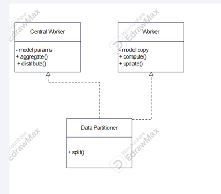
Code Problem - Distributed Training Concept Simulator

This C++ program is a simple multithreaded demonstration of the Distribution Strategy design pattern used in distributed machine learning systems. It conceptually shows how a CentralServer coordinates with multiple Workers to perform parallel tasks without involving any mathematical computations. The DataPartitioner divides a total workload (e.g., data batches) among workers, the CentralServer broadcasts a model version to all workers, and each Worker runs in its own thread, "processing" its assigned batches by sleeping briefly to simulate work before sending a completion signal back to the server. The server collects these acknowledgements, aggregates them, and increments the model version for the next round—illustrating the key steps of distribute, parallel process, aggregate, and update.
Worker.h,
DataPartitioner.h,
CentralServer.h,
DistTraining.cpp.

What it demonstrates:

• Broadcast: Central sends a version (think “parameters”) to all workers.
• Parallel work: Workers process their assigned mini-batches concurrently.
• Collect/Aggregate: Central collects simple DONE signals and “updates” by bumping the version.
• Iterate: Repeat for a few rounds to show the strategy loop.

Distribution Strategy vs Parallel Processing

1. Core Idea

2. Goal and Context

3. Communication Model

4. Typical Example

• Parallel Processing Example: A program uses threads to process 10 files at once, each counting words independently.
• Distribution Strategy Example: A deep learning job uses 4 GPUs, each processing a mini-batch and averaging gradients to keep models synchronized.

5. Analogy

Parallel processing = many chefs cooking different dishes independently.

Distribution strategy = many chefs cooking parts of the same dish, constantly sharing ingredients and results.

6. Summary