Week 10 - Patterns that Modify Model Training: Hyperparameter Tuning Patterns. Resilience Patterns: Stateless Serving Function and Batch Serving

Lecture recording here.

Lab recording here.

Introduction

This week we will look at another pattern that modifies model training: the hyperparameter tuning pattern. The hyperparameter tuning pattern inserts the training loop into an optimization method to find the optimal set of model hyperparameters.

We will also look at two resilience patterns: stateless serving function and batch serving. The stateless serving function pattern exports the machine learning model as a stateless function so that it can be shared by multiple clients in a scalable way. This is because production machine learning systems must be able to synchronously handle thousands to millions of prediction requests per second. The batch serving resilience design pattern focuses on ensuring the reliability and fault tolerance of batch processing systems. This pattern is particularly important in scenarios where large volumes of data are processed in scheduled batches, and any failure can result in significant delays or data loss.

Videos

Assignment(s)

Assignment 5 - Multimodal Input: An Autonomous Driving System

The Hyperparameter Tuning Design Pattern

A Machine Learning model is defined as a mathematical model with a number of parameters that need to be learned from the data. By training a model with existing data, we are able to fit the model parameters. However, there is another kind of parameter, known as Hyperparameters, that cannot be directly learned from the regular training process. They are usually fixed before the actual training process begins. These parameters express important properties of the model such as its complexity or how fast it should learn. For more information see Hyperparameter Tuning - Brief Theory and What you won't find in the HandBook.

The Rationale

The rationale behind the Hyperparameter Tuning Design Pattern is to systematically explore different combinations of hyperparameter values to identify the configuration that produces the best results. By tuning the hyperparameters, we aim to improve the model's performance, generalization, ability, and robustness.

The UML

Here is the UML diagram for the hyperparameter tuning design pattern:

  ----------------------------------
  |    Hyperparameter Tuning       |
  |    Design Pattern              |
  ----------------------------------
  |                                |
  | + Define hyperparameters       |
  | + Define search space          |
  | + Define evaluation metric     |
  | + Select tuning strategy       |
  | + Train and evaluate models    |
  | + Select best hyperparameters  |
  | + Test the model               |
  ----------------------------------
 

1. Define the hyperparameters: Identify the hyperparameters that need to be tuned. Examples of common hyperparameters include learning rate, batch size, regularization strength, number of hidden units, and kernel size.
2. Define the search space: Determine the range or set of values for each hyperparameter that will be considered during the tuning process. This search space can be defined manually or automatically using techniques like grid search, random search, or Bayesian optimization.
3. Define the evaluation metric: Select an appropriate metric to evaluate the performance of the model. This could be accuracy, precision, recall, F1 score, or any other relevant metric depending on the problem domain.
4. Select a tuning strategy: Choose a strategy to explore the hyperparameter search space. Some common strategies include grid search, random search, and more advanced methods like Bayesian optimization, genetic algorithms, or gradient-based optimization.
5. Train and evaluate models: Train and evaluate a series of models with different hyperparameter configurations using cross-validation or a separate validation set. The evaluation metric defined earlier is used to compare and rank the performance of different models.
6. Select the best hyperparameters: Identify the hyperparameter configuration that achieved the best performance according to the evaluation metric. This configuration is typically selected as the final set of hyperparameters for the model.
7. Test the model: Finally, evaluate the model's performance on an independent test set using the selected hyperparameters to estimate its real-world performance.

Code Example - Hyperparameter Tuning

In this program, we demonstrate each step of the Hyperparameter Tuning Design Pattern.
We define the hyperparameters (learningRate, numHiddenUnits, regularizationStrength) in Step 1.
We define the search space for each hyperparameter (learningRates, hiddenUnits, regularizationStrengths) in Step 2.
The evaluation metric is the mean squared error (MSE) in this example, defined as bestMetric in Step 3.
We use nested loops to iterate over the search space of each hyperparameter in Step 4, representing the tuning strategy (in this case, grid search).
Within the loops, we train and evaluate the model using the current hyperparameters in Step 5. The evaluation metric (MSE) is calculated by the trainAndEvaluateModel function.
We select the best hyperparameters based on the metric value in Step 6. If the current metric is better than the previous best, we update the best hyperparameters and metric.
Finally, in Step 7, we print the best hyperparameters and the corresponding metric.
C++: Tuning.cpp.
C#: Tuning.cs.
Java: Tuning.java.
Python: Tuning.py.

Common Usage

The hyperparameter tuning pattern is widely used in the software industry for optimizing the performance of machine learning models and algorithms. The following are some common usages of the hyperparameter tuning pattern:

1. Model Selection: Hyperparameter tuning is used to select the best set of hyperparameters for a given machine learning model. By systematically exploring different combinations of hyperparameters, practitioners can identify the configuration that yields the best performance on a validation set or through cross-validation.
2. Algorithm Optimization: Hyperparameter tuning is employed to optimize the parameters of machine learning algorithms. For example, in gradient boosting algorithms like XGBoost or LightGBM, hyperparameters such as the learning rate, number of estimators, and maximum depth of trees can significantly impact the algorithm's performance. Tuning these hyperparameters helps achieve the best trade-off between accuracy and computational efficiency.
3. Neural Network Training: Hyperparameter tuning is crucial for training deep neural networks. Parameters such as learning rate, batch size, optimizer settings, and regularization techniques play a critical role in achieving good training convergence and preventing overfitting. Tuning these hyperparameters helps improve the model's generalization capabilities.
4. Feature Selection: Hyperparameter tuning is used to optimize the selection of features in machine learning pipelines. By exploring different subsets of features or applying feature selection algorithms, practitioners can identify the most relevant features that contribute to the model's performance.
5. Reinforcement Learning: Hyperparameter tuning is employed to optimize the hyperparameters of reinforcement learning algorithms, such as exploration-exploitation trade-offs, learning rates, discount factors, and exploration policies. Tuning these hyperparameters can lead to better convergence and more efficient learning in reinforcement learning tasks.
6. Time Series Forecasting: Hyperparameter tuning is used to optimize hyperparameters in time series forecasting models, such as the number of lagged variables, window sizes, and regularization parameters. Tuning these hyperparameters can improve the model's bility to capture temporal dependencies and make accurate predictions.

Code Problem - F1 Score

This code demonstrates the generation of the F1 score using the hyperparameter tuning design pattern. Here's a step-by-step explanation of the code:

1. The generateDataset function generates a synthetic binary classification dataset. It randomly generates samples with two features x and y and assigns labels based on whether x + y >= 0 or not.
2. The trainAndEvaluateSVM function trains and evaluates an SVM model using the given dataset and hyperparameters C and gamma. In this example, the function calculates the F1 score as the evaluation metric based on accuracy. It counts the true positives, false positives, and false negatives by comparing the predicted labels with the actual labels of the dataset.
3. The main function is the entry point of the program. It follows the hyperparameter tuning design pattern using the grid search strategy.
   • Step 1: Define the hyperparameters C and gamma.
   • Step 2: Define the search space for hyperparameters using vectors Cs and gammas.
   • Step 3: Define the evaluation metric as the best F1 score found so far, initialized to the lowest possible value, and variables to store the best hyperparameters.
   • Step 4: Select the tuning strategy, which is a nested loop for grid search. It iterates over all combinations of C and gamma values.
   • Step 5: Train and evaluate SVM models using the current hyperparameters from the search space. It calls the trainAndEvaluateSVM function and passes the generated dataset along with the current C and gamma values.
   • Step 6: Select the best hyperparameters based on the F1 score. If the current F1 score is higher than the best F1 score found so far, update the best F1 score and store the corresponding C and gamma values.
   • Step 7: Print the best hyperparameters (C and gamma) and the best F1 score.

Code Example - Support Vector Machine Classification

Below is a complex example of the Hyperparameter Tuning Design Pattern using a hypothetical scenario of a support vector machine (SVM) for classification:
MLModel.h,
SVMClassifier.h,
HyperparameterTuningStrategy.h,
RandomSearchStrategy.h,
GridSearchStrategy.h,
HyperparameterTuningContext.h,
SVMMain.cpp.

The Stateless Serving Function Design Pattern

The Rationale

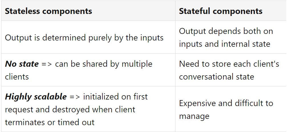
The rationale behind the stateless serving function design pattern is to enable scalable and efficient handling of incoming requests in a distributed computing environment. In this pattern, each request is treated independently, and the server functions do not maintain any state or store any context about previous requests. Instead, they focus solely on processing the current request and generating a response.

When we implement the stateless design pattern, we create classes and objects that do not retain state changes. In this approach, each use of the object, as an example, uses the object in its organic form. In our context, state refers to the values of the object's variables. So, there is no definitive list of states. The state of an object is specific to a moment in time. Using this design pattern, we can have a production ML system synchronously handle millions of prediction requests per second.

For a discussion on stateful vs stateless, see RedHat: Stateful vs stateless.

The UML

Here is the UML diagram for the stateless serving function pattern:

  +-----------------+
  |   Application   |
  +-----------------+
  | + serve(request)|
  +-----------------+
          |
          V
  +--------------------+
  |  RequestProcessor  |
  +--------------------+
  | - process(request) |
  +--------------------+
          |
          V
  +-------------------+
  |     Controller    |
  +-------------------+
  | - handle(request) |
  +-------------------+
          |
          V
  +------------------+
  |    Business      |
  +------------------+
  | - doSomething()  |
  +------------------+  

1. Application: The Application class represents the server application. It has a serve() function that takes a Request object and passes it to the RequestProcessor.
2. RequestProcessor, Controller: The RequestProcessor class handles the processing of the request and invokes the Controller to handle the business logic.
3. Business: The Business class contains the actual business logic that needs to be performed.

Code Example - Stateless Serving Function Pattern

This example is code representation of the above UML:
C++: Stateless.cpp.
C#: Stateless.cs.
Java: Stateless.java.
Python: Stateless.py.

Common Usage

The following are some common usages of the stateless serving function pattern:

1. Microservices architecture: Stateless serving functions are often used in microservices-based architectures. Each microservice can be implemented as a stateless function, focusing on a specific functionality or business logic. This enables independent scaling and deployment of microservices, making it easier to manage and update individual components of a complex system.
2. RESTful APIs: Stateless serving functions are well-suited for building RESTful APIs. Each API endpoint can be implemented as a separate function, handling incoming requests independently. This allows for horizontal scaling and efficient resource utilization, especially when the API experiences varying levels of traffic. Stateless functions are also compatible with popular API gateway services and can be easily integrated into API management platforms.
3. Web applications: Stateless serving functions can power server-side logic in web applications. They can handle incoming requests, process data, and generate responses without the need for maintaining server-side sessions or shared state. This enables efficient scaling and distribution of web application workloads while maintaining responsiveness and minimizing resource usage.
4. Event-driven systems: Stateless functions are frequently used in event-driven architectures and systems that process real-time events or messages. They can be triggered by events such as messages from message queues, updates in data streams, or events from external systems. Stateless functions process these events independently, allowing for scalability and parallel processing of events.
5. Data processing pipelines: Stateless serving functions are suitable for building data processing pipelines, especially in scenarios involving batch processing or stream processing. Each function can perform a specific data transformation or analysis task, allowing for efficient parallel processing of data. By chaining multiple functions together, complex data processing pipelines can be constructed and scaled as needed.
6. Serverless computing: Stateless serving functions are a fundamental building block of serverless computing platforms. In serverless architectures, functions are executed in response to specific events or triggers, and resources are allocated dynamically. By utilizing stateless functions, developers can focus on writing the business logic without worrying about infrastructure management or scalability.
7. Machine learning inference: Stateless serving functions are used for serving machine learning models in production. When a prediction request comes in, the function loads the required model, performs the inference, and returns the prediction. This allows for efficient scaling and parallel execution of predictions, ensuring that the system can handle high volumes of requests.

Code Problem - Server Handler

In this example, a server application handles multiple types of requests using a stateless serving function design pattern. The Request class represents a request made to the server and provides a method to retrieve the request details. The Business class simulates processing the request by performing some business logic based on the request. In this example, it simply prints the request. The Controller class handles the request and delegates it to the Business class for processing. The RequestProcessor class maintains a mapping of endpoints to their respective controllers. It extracts the endpoint from the request and finds the corresponding controller to handle the request. The Application class serves as the entry point of the program. It allows registering controllers for specific endpoints and processes incoming requests.

In the main() function, we create an instance of the Application class and register two controllers for different endpoints. We then create multiple requests and pass them to the serve() method of the application, which delegates the processing to the appropriate controller based on the request's endpoint. When you run this program, you will see the requests being processed by the respective controllers based on their endpoints. If an invalid endpoint is provided, an error message will be displayed.
Request.h,
Business.h,
Controller.h,
RequestProcessor.h,
RequestProcessor.cpp,
Application.h,
Server.cpp.

Code Problem - Socket Based Server

Sample code for a simple socket-based server for handling requests is given below. This version uses Winsock for socket programming on Windows. Note that you'll need to link against the Ws2_32.lib library.
MLModel.h,
StatelessServingFunction.h,
RequestHandler.h,
RequestHandler.cpp,
Server.h,
Server.cpp,
ServerMain.cpp.

The Batch Serving Design Pattern

The batch serving design pattern focuses on the efficient and reliable processing of large volumes of data in scheduled batches, rather than in real-time. This pattern is commonly used in data processing pipelines for tasks such as ETL (Extract, Transform, Load), data warehousing, and offline machine learning model training.

The Rationale

The batch serving design pattern enables efficient, scalable processing of large data volumes by scheduling and distributing workloads across multiple nodes, optimizing resource utilization and minimizing costs. It enhances reliability and fault tolerance through robust error handling mechanisms, ensuring data consistency and integrity. Additionally, batch processing simplifies data pipeline management, testing, and debugging compared to real-time systems. It is particularly suited for use cases like ETL processes, analytics, reporting, and machine learning model training.

The UML

The following is a very primitive diagram of the batch serving design pattern.

  +-----------------------------------------------+
  |                    Data Source                |
  +-----------------------------------------------+
                     |
                     v
  +-----------------------------------------------+
  |                 Data Ingestion                |
  |  - Collect data from various sources          |
  |  - Store in centralized repository            |
  +-----------------------------------------------+
                     |
                     v
  +-----------------------------------------------+
  |          Job Scheduler (e.g., Airflow)        |
  |  - Manage and orchestrate batch jobs          |
  |  - Schedule jobs at regular intervals         |
  +-----------------------------------------------+
                     |
                     v
  +-----------------------------------------------+
  |         Batch Processing Framework            |
  |        (e.g., Hadoop, Spark)                  |
  |  - Distribute data processing                 |
  |  - Ensure fault tolerance and scalability     |
  +-----------------------------------------------+
                     |
                     v
  +-----------------------------------------------+
  |            Data Transformation                |
  |  - Clean, normalize, and aggregate data       |
  |  - Apply business logic                       |
  +-----------------------------------------------+
                     |
                     v
  +-----------------------------------------------+
  |               Output Storage                  |
  |  - Store processed data for consumption       |
  |  - Use suitable data stores                   |
  +-----------------------------------------------+
                     |
                     v
  +-----------------------------------------------+
  |      Monitoring and Logging                   |
  |  - Track job performance                      |
  |  - Log execution details and errors           |
  +-----------------------------------------------+
                     |
                     v
  +-----------------------------------------------+
  |      Fault Tolerance and Recovery             |
  |  - Implement retry logic                      |
  |  - Use checkpointing                          |
  |  - Ensure idempotent operations               |
  +-----------------------------------------------+

Code Example - Batch Serving

Here is a simple example to demonstrate the batch serving design pattern. In this example, we'll simulate a scenario where we process a batch of numbers by squaring each number in the batch.
C++: BatchServing.cpp.
C#: BatchServing.cs.
Java: BatchServing.java.
Python: BatchServing.py.

Common Usage

The batch serving design pattern is commonly used in various domains and applications where processing multiple requests or tasks in groups (batches) can significantly improve efficiency, reduce latency, and optimize resource utilization. Here are some common areas where this pattern is employed:

1. Data Processing and ETL (Extract, Transform, Load) Pipelines: Used in data warehousing and big data processing to handle large volumes of data efficiently. Batches of data are extracted from sources, transformed, and loaded into storage systems.
2. Machine Learning and AI: Training machine learning models often involves processing data in batches to improve performance and convergence. Inference and prediction tasks can also benefit from batch processing, where predictions for multiple inputs are made in one go.
3. Database Operations: Bulk inserts, updates, and deletes in databases can be optimized by batching operations to reduce the number of transactions and improve throughput. Batch queries can also be used to retrieve large datasets more efficiently.
4. Network Communications: Reduces the overhead of network latency by sending and receiving data in batches rather than individually. Common in APIs, message queues, and other client-server communications.
5. File Processing: Large files can be processed in smaller chunks or batches to manage memory usage and improve performance. Common in log file analysis, video processing, and other file-based operations.
6. Financial Transactions: Batch processing is used for handling large numbers of transactions, such as in banking and stock trading systems. Helps in reducing the processing time and improving reliability.
7. Email and Notification Systems: Sending emails or notifications in batches can help manage load and avoid spamming servers. Often used in marketing campaigns and alert systems.
8. Image and Video Processing: Tasks such as resizing, filtering, and encoding can be performed on batches of images or video frames. Improves efficiency in multimedia applications.
9. Distributed Systems and Cloud Computing: Batch processing frameworks like Apache Hadoop, Apache Spark, and Google Cloud Dataflow are designed to handle large-scale data processing tasks. Commonly used for data analytics, batch processing jobs, and ETL processes.
10. Web Applications: Batch processing is used for tasks such as data aggregation, reporting, and background jobs. Frameworks like Celery (Python), Sidekiq (Ruby), and others facilitate batch job processing.

Code Problem - Batch Prediction

This example perform batch predictions using a linear regression model: BatchPrediction.cpp.
data is defined as a constant vector of vectors of doubles. This represents our dataset directly in the code.
The LinearRegression class represents a simple linear regression model.
The model is initialized with a vector of coefficients and an intercept.
The predict() method makes a prediction for a single feature vector.
The batchPredict() method makes predictions for a batch of feature vectors.

Microchip Route and Place (out of scope)

For a discussion of machine learning applied to the very difficult problem of routing and placing digital electronic components on a micro-chip, see Route and Place.