Assignment 1 - Analog Circuit Simulator
Due - Sunday, October 26, 2025
This is a group project of 2 or 3 students per group. The groups can be found in the document
Assignment1_Groups.docx.
Use-Case Scenario
Work on an analog circuit simulator (ANASIM) has been started by a former employee and you are asked to take over. You must
consider the theoretical background of the work, and the completion of the design and implementation that was in progress.
You also have to come up with a project plan, which has not even been started. Included in the project plan is the scheduling,
cost estimation (assume $50 per person-hour), and quality assurance. As you are going through the work, you
might see things you do not like, but you do not have the time to implement those changes. Once this product has been
released (version 1.0), you will have the opportunity (in Lab 4) to suggest and implement those changes for
release version 2.0.
Introduction
Theoretical Background
There are three approaches to analog circuit simulation: numerical methods, machine learning, and heuristic algorithms. Each is described below.
Numerical Methods for the Solution of Analog Electronic Circuits
Simulation is a very important part of design. Most hardware projects undergo rigorous simulations before
implementation actually occurs. Simulating the behaviour of an analog circuit can be quite simple. One can
simply obtain the differential equation for the circuit, and use well known numerical methods to solve them.
Several numerical algorithms are well know. Below is a summary of a few:
- Euler's method. The Euler method (also called forward Euler method) is a first-order numerical procedure
for solving ordinary differential equations with a given initial value. It is the most basic explicit
method for numerical integration of ordinary differential equations. The Euler method is a first-order method,
which means that the local error (error per step) is proportional to the square of the step size, and the global
error (error at a given time) is proportional to the step size. The Euler method often serves as the basis to
construct more complex methods. One way to think about Euler's method is that it uses the
derivative at the current solution point (t0, u0) to create a linear prediction of the solution at the next time t1.
- Midpoint method. The midpoint method tries for an improved prediction over the Euler's method. It does this
by taking an initial half step in time, sampling the derivative there, and then using that forward information as the slope.
In other words, it replaces the tangent line by a line that is starting to bend correctly.
- Runge-Kutta method. One of the standard workhorses for solving ordinary differential equations is the called the Runge-Kutta
method. This method is simply a higher order approximation to the midpoint method. Instead of shooting to the midpoint, estimating
the derivative, the shooting across the entire interval - the Runge-Kutta method, in a sense takes, four steps, shooting
across one quarter of the interval, estimating the derivative, then shooting to the midpoint, and so on. The precise
manner in which the method propagates across a time step is done in the optimal way for the four steps
For more details, see the publication Numerical Methods for Differential Equations.
The problem of applying well known numerical methods to solving analog electronic circuits is that these methods assume
linear behaviour. The key point that distinguishes a nonlinear circuit from a linear circuit is the relationship between
the input and output signal. If you graph the output signal versus the input signal for a linear circuit, then the graph
will be a straight line for all input signal levels. With a nonlinear circuit, the output will not be a straight line.
Instead, the output will be a curve.
It is likely that all the circuits you built were linear circuits, meaning they only contained resistors, capacitors, and non-ferritic
inductors. While this is a great way to get an important introduction into the fundamentals of basic circuits, almost all modern
circuits contain many more complicated elements and functionality. For a discussion of linear and nonlinear circuits, see
The Basics of Linear vs. Nonlinear Circuits.
To summarize, linear devices include resistors, capacitors, and most inductors when driven with low current.
Nonlinear devices include semiconductor devices (transistors and diodes), ferrite inductors driven at high
current where magnetic saturation occurs, all amplifiers, and almost all integrated circuits. Therefore, for
non-linear circuits, we cannot rely on numerical methods and we have to take another approach.
The Machine Learning Cost Function
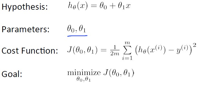
The machine learning cost function attempts to approximate real data with a hypothetical equation. Let us say we
wish to approximate data with a first order function:
hθ(x) = θ0 + θ1 x
The parameters we want to guess are θ0 and θ1. We generate a cost function that determines the difference
between actual data and this approximation by taking the square of the difference between the points. We choose
θ0 and θ1 to minimize this difference. This is summarized below:
It is possible to apply the machine learning cost function to non-linear electronic circuits if we expand
hθ(x) to a much higher order equation. For instance:
hθ(x) = θ0 + θ1 x + θ2 x2 + θ2 x3 ...
You will notice that this cost function is similar to the Taylor Series,
which attempts to approximate any mathematical function as a series of exponents and coefficients.
We could apply voltages to the circuits and measure the currents we seek, determine the optimum θ's, and use that to predict behaviour.
Heuristic Algorithms for the Solution of Analog Electronic Circuits
A heuristic algorithm is one that is designed to solve a problem in a faster and more efficient fashion than traditional methods by sacrificing
optimality, accuracy, precision, or completeness for speed. Heuristic algorithms are often used to solve NP-complete problems, a class of
decision problems. In these problems, there is no known efficient way to find a solution quickly and accurately although solutions can be
verified when given. Heuristics can produce a solution individually or be used to provide a good baseline and are supplemented with optimization
algorithms. Heuristic algorithms are most often employed when approximate solutions are sufficient and exact solutions are necessarily computationally
expensive.
For a linear electronic circuit, a heuristic algorithm is not required, since all voltages and currents through the circuit can be solved using
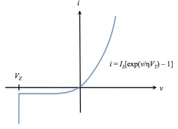
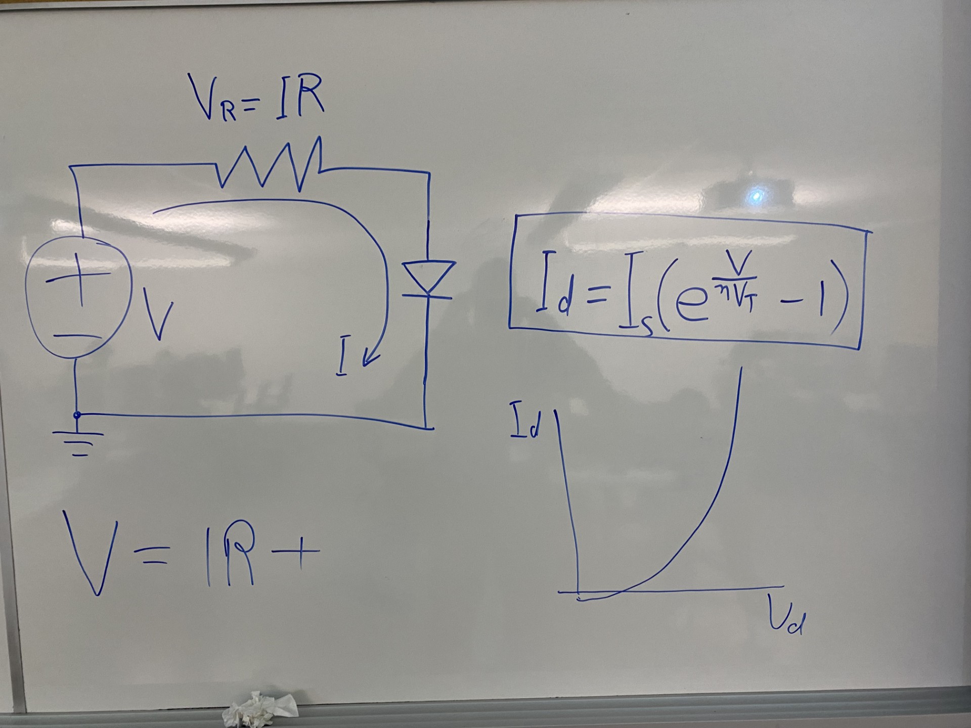
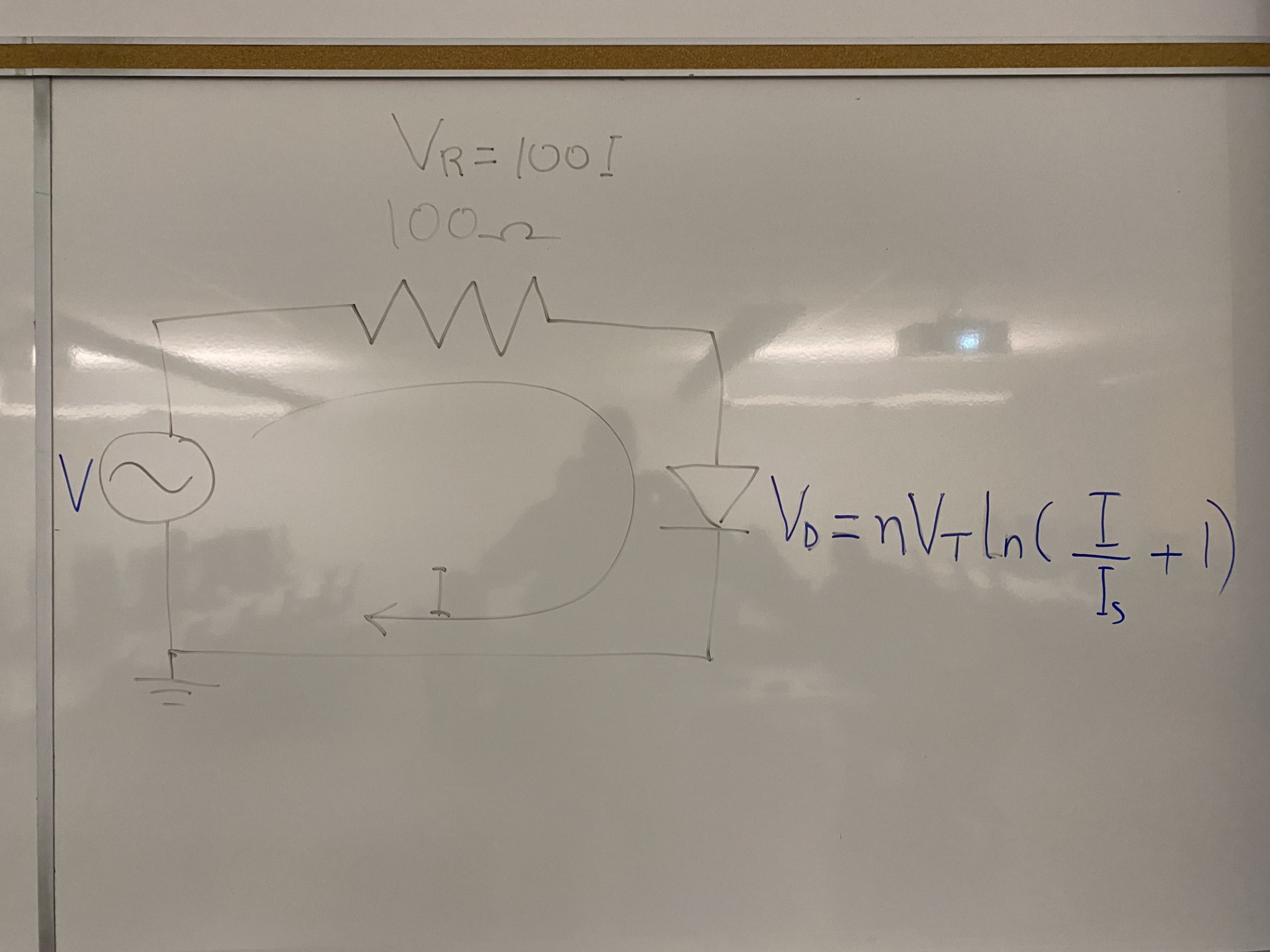
numerical analysis. For non-linear circuits, a heuristic approach is required. Consider the diode. The voltage current relationship is given as:
i(v) = IS[e(v/(ηVT))-1], v>VZ
where IS is the reverse saturation current,
v is the applied voltage (reverse bias is negative),
VT=T/11,586 is the volt equivalence of temperature, and
η is the emission coefficient, which is 1 for germanium devices and 2 for silicon devices.
Note that for v≤VZ, the diode is in breakdown and the ideal diode no longer applies.
The ideal diode i-v characteristic curve is shown below:
Sometimes the inverse relation is more useful, and that is the voltage across a diode as a function of the current:
v(i) = ηVTln[(i/IS)+1]
There are many other non-linear circuit components. For instance, the transistor, the operational amplifier, any magnetic circuit where magnetic
saturation occurs. In fact, such simple components such as the resistor, capacitor and inductor exhibit non-linear behaviour if they are pushed
to their limits.
The Work Breakdown
There are several parts to assignment 1. First is the cost function with a heuristic algorithm, which is used to guess the current for a particular
instant in time within a tolerance. The second are the circuit components, the third is the graphics.
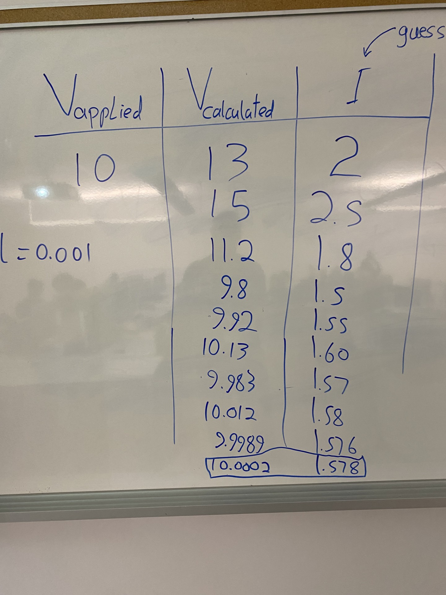
The Cost Function
Assignment 1 revolves around a cost function. This is a function that tries to predict the currents of the components given
the applied voltage. The cost function sums the voltages of the components and compares to the applied voltage. The "cost" is the
difference between the applied voltage and the sum of the voltages across the components. Several iterations are taken until the cost
is below a tolerance level, which is typically very low. The following variables are used:
- I1 is the predicted current. Several iterations are required to approach the correct current.
- J1 is the cost of the function for the current iteration. We try to reduce this to zero or close to zero.
- J0 is the cost of the function for the previous iteration. We use both J1 and J0 to predict the current.
- voltage is the voltage applied across the circuit.
- sumVoltage is the voltage summed across all component for a given current I1.
As you can see from the above, the idea is to repetitively guess I1 such that the cost J1 (sumVoltage-voltage) approaches zero.
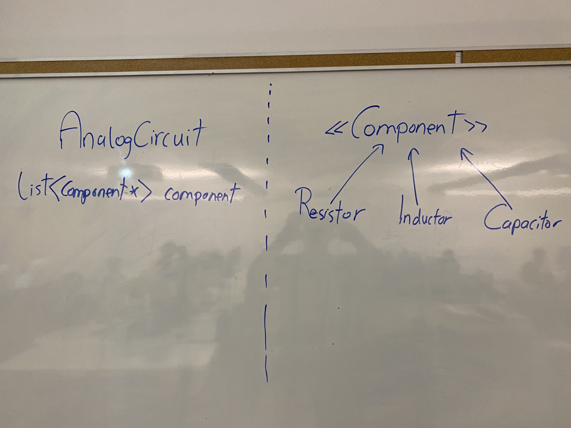
The Circuit Components
Some files have been given to you. You can change these. The component class, which acts as a base class for all circuit components,
is given to you. You will have to implement code for the resistor, capacitor and inductor. All these are derived from the component
class. Each component will display its current in a different colour, and each component has a name. There are pure virtual
functions which require implementation in derived classes. The header file for the analog circuit has been given to you. This class
contains a list of circuit components, a static display function which can be called from all of its components, a run function for
when you want to run the actual simulation, the cost function as described above, and a destructor. Some function implementations
have been given in the CPP file for the analog circuit. Finally, a main function has been provided in full. See all files at:
Component.h, (complete)
AnalogCircuit.h, (complete)
AnalogCircuit.cpp (incomplete) and
AnalogCircuitMain.cpp (complete).
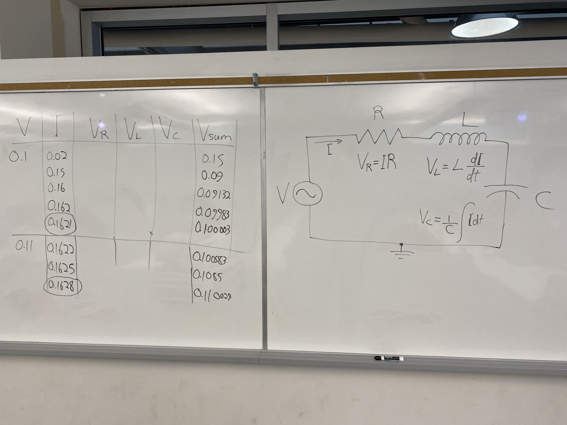
The analog circuit used in this assignment does not have non-linear components, but can be used to verify the functionality of your software. We will
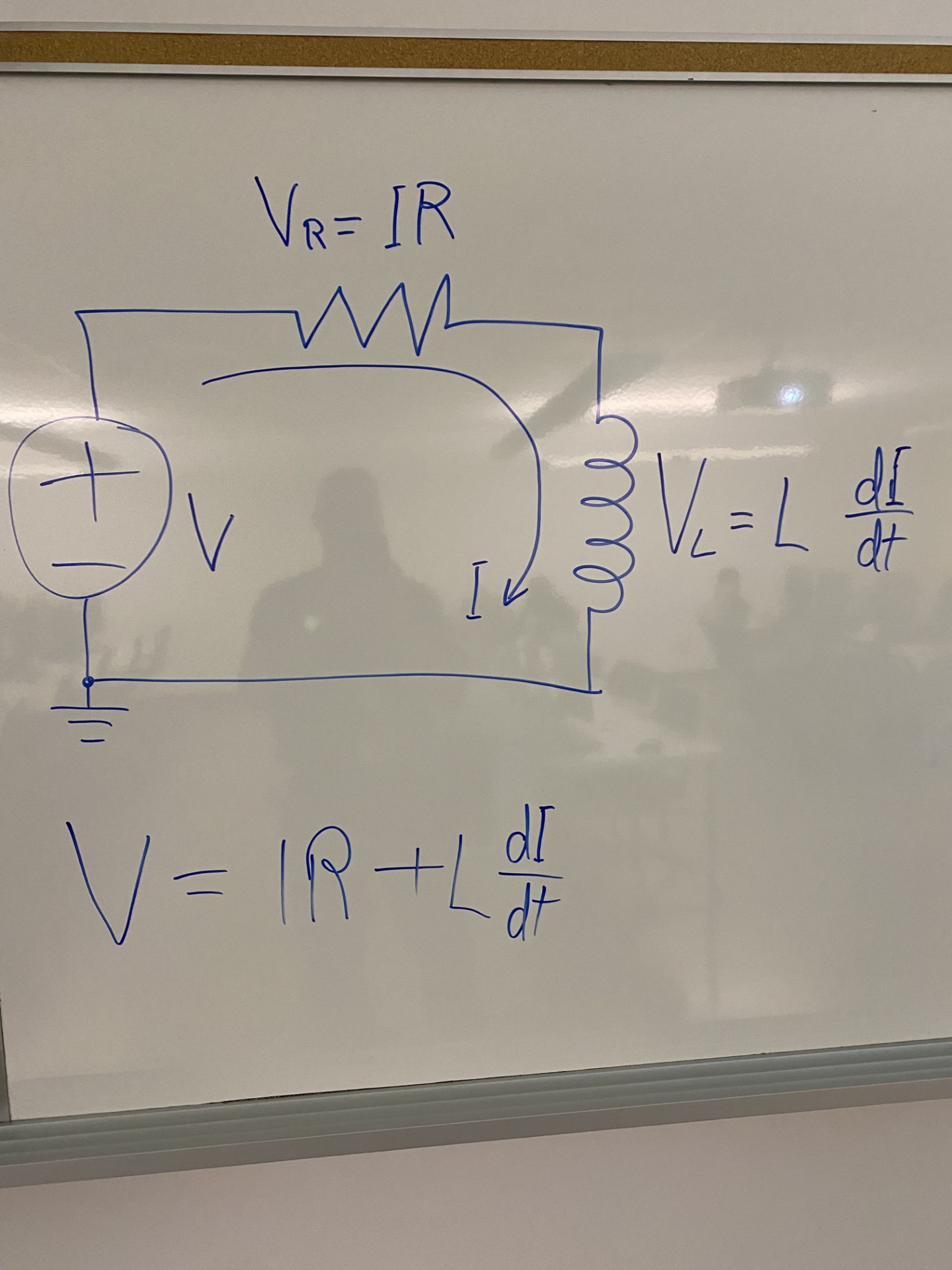
apply a sinusoidal voltage for 0.6 seconds, then 0 volts for the remainder of the simulation. The circuit looks as follows:
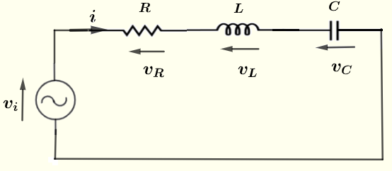
Recall from your physics and electronics classes, the voltages as a function of current across these components are as follows:
- Resistor: VR(t) = i R
- Inductor: VL(t) = L di/dt
- Capacitor: VC(t) = V0 + 1/C ∫i dt
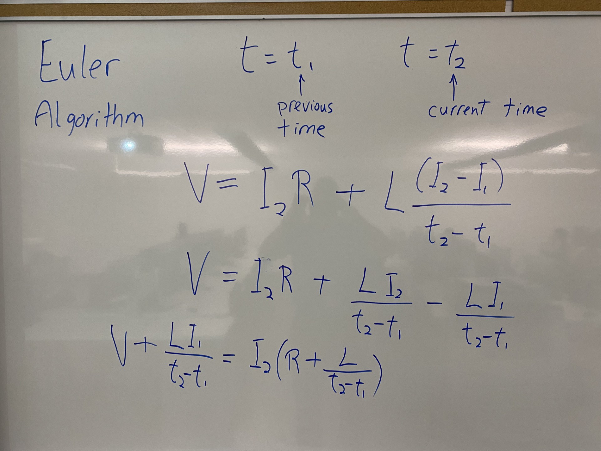
By using a small time-step, the above equations can be approximated using Euler's method as follows:
- The Resistor. The resistor has a resistance in Ohms as well as a current running through it. The voltage across a resistor is simply
the current going through the resistor times the resistance:
voltage = current * resistance.
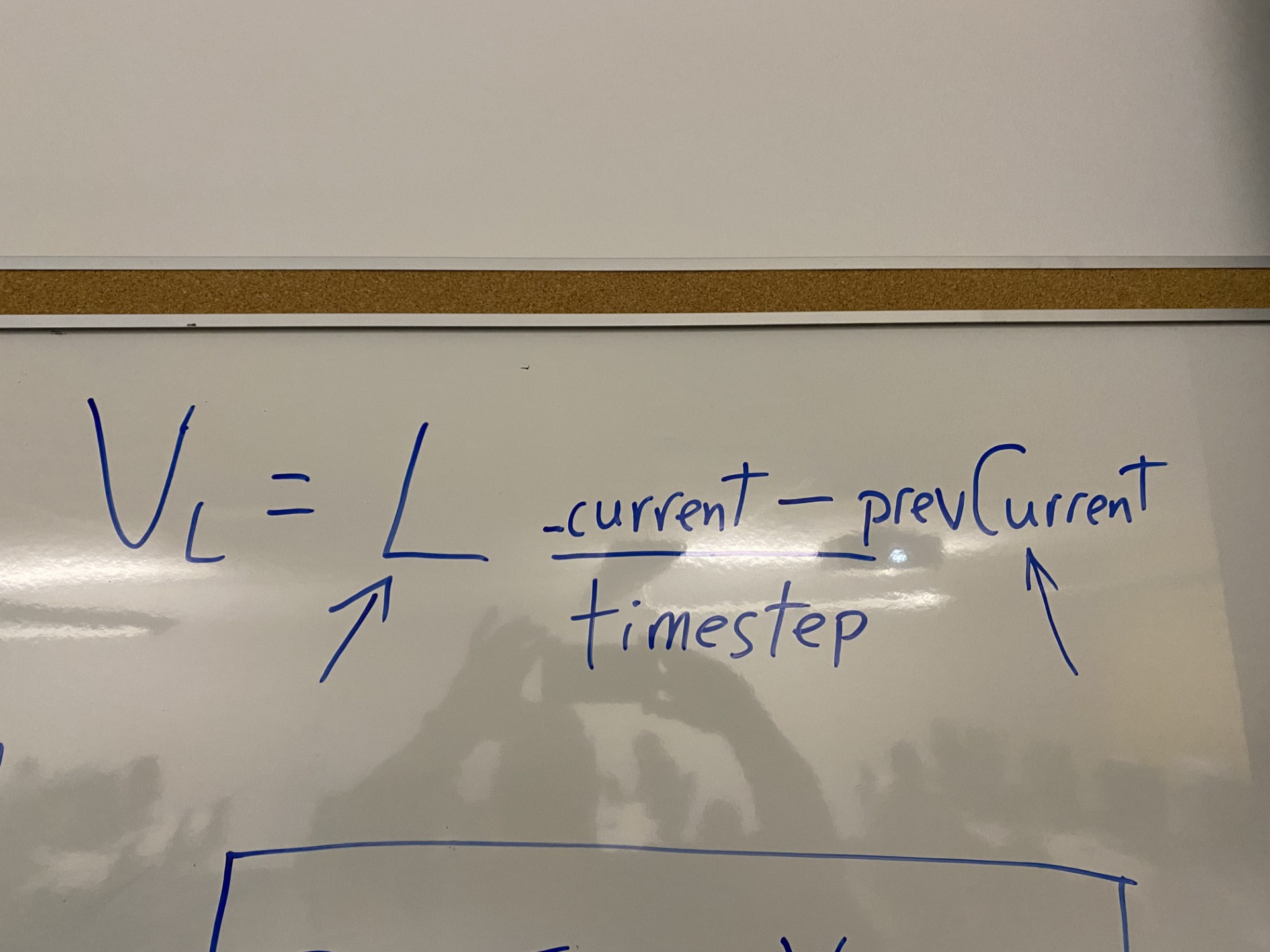
- The Inductor. An inductor has an inductance in Henries and has current running through it in Amperes. If a current is applied to the inductor,
the voltage across the inductor is given as follows:
voltage = inductance * (current[1] - current[0]) / timestep, where
current[1] is the applied current and current[0] is the current from the
previous time step.
Once the correct current has been determined, don't forget to update your
current: current[0] = current[1].
- The Capacitor. The capacitor has a capacitance in Farads, a current running through it in Amperes, and a voltage stored in it in Volts. If a current is
applied to the capacitor, the voltage across the capacitor is as follows:
voltage[1] = voltage[0] + current * timestep / capacitance, where
voltage[1] is the current voltage and voltage[0] is the voltage from the
previous time step.
Once the correct current has been determined, don't forget to update your
voltage: voltage[0] = voltage[1].
The Graphics
The graphics library suggested for this assignment is OpenGL. The following link explains how to add OpenGL to Visual Studio:
Configuring Visual Studio for OpenGL Development.
To summarize:
- Create a project.
- Right-click on "References", then click on Manage Nuget Packages.
- Select Package Manager Console.
- Click on the prompt (where it says PM), and type: Install-Package nupengl.core Then press enter.
A manual of OpenGL API's can be found at:
OpenGL API Documentation Overview.
Summary of Tasks
In this assignment, you have to plot the applied voltage as well as the voltages across each component.
A sample run with a 50Hz sinusoid with 10V zero-to-peak with window width of 1000, window height of 500 and a scaling factor of
1.2 can be shown with the below graphic:
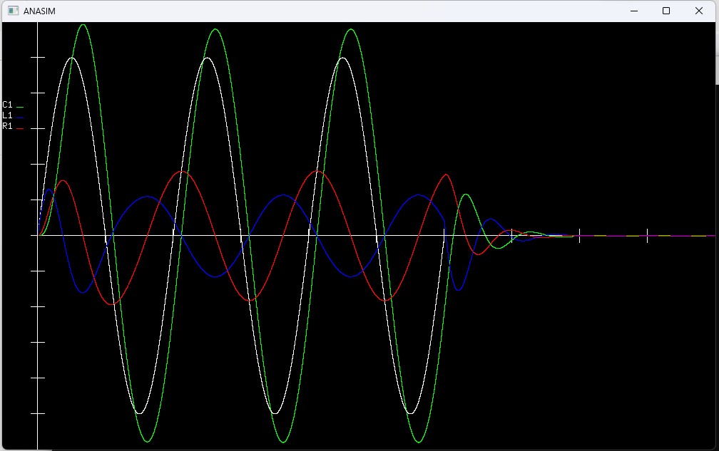
The output file can be seen at: RLC.dat.
For this assignment, you must complete the following tasks and answer the following questions:
- You must provide a project plan by Wednesday, October 8th.
In this project plan be sure to include a schedule, a cost estimation based on $50 per
person-hour as well as a quality assurance plan to ensure reliable software.
- You must provide a working prototype by Wednesday, October 8th.
- The project consists of three parts. You must have all parts working by the end of the assignment.
- Familiarize yourself with the graphics library.
- Complete the classes for the Inductor, Capacitor and Resistor.
- Complete the function implementations of the AnalogCircuit class.
The questions comprise a large portion of this assignment. Here you must show me that you can analyze the project and make suggestions for improvements.
- You may notice that the cost function is based on Euler's method. What other method(s) might be applied to enable it to run more efficiently?
- You may notice that the cost function has no intelligence. It does not learn. This heuristic algorithm does not comply
with the principles of machine learning. How might you add intelligence to our cost function to enable it to run more efficiently?
- Devise a completely different way to implement the cost function. Is there some quicker way of guessing the present current knowing the previous voltage and current?
- You may not like the way this project was designed and implemented. What changes would you suggest and why (ie. graphics, circuit components, using C++, ...).
Marking Rubric
Note that this assignment partially fulfills two of the
Canadian Engineering Accreditation Board
graduate attributes that our engineering graduates should have:
- Design (DE.5),
- Economics & Project Management (EP.2).
Both attributes are assessed here.
Assignment 1 is worth 20% of your final grade and as such is marked out of 20 as follows:
| Does not meet expectations | Satisfactory | Good | Exceeds Expectations |
|---|
The Project Plan
(3 marks) EP.2 | Does not meet requirements | Meets the most important requirements | Meets all requirements with minor errors | Meets all requirements with no errors |
The Prototype
(2 mark) DE.5 | Does not meet requirements | Meets the most important requirements | Meets all requirements with minor errors | Meets all requirements with no errors |
The Graphics Library
(3 marks) DE.5 | Does not meet requirements | Meets the most important requirements | Meets all requirements with minor errors | Meets all requirements with no errors |
The Component Classes
(3 marks) DE.5 | Does not meet requirements | Meets the most important requirements | Meets all requirements with minor errors | Meets all requirements with no errors |
The Analog Circuit Class
(3 marks) DE.5 | Does not meet requirements | Meets the most important requirements | Meets all requirements with minor errors | Meets all requirements with no errors |
Code Documentation
(2 mark) | Does not contain documentation | Contains header documentation for either all files or for all functions within each file |
Contains header documentation for all files and for most functions within each file | Contains header documentation for all files and for all functions within each file.
Documents unclear code. |
Questions
(4 marks) | Answers no question correctly | Answers some questions correctly |
Answers most questions correctly | Answers all Questions correctly |
Submission
Please email all source code and answers to questions to:
miguel.watler@senepolytechnic.ca
Your answers to questions can be submitted in a separate document or embedded within your source code.
Late Policy
You will be docked 10% if your assignment is submitted 1-2 days late.
You will be docked 20% if your assignment is submitted 3-4 days late.
You will be docked 30% if your assignment is submitted 5-6 days late.
You will be docked 40% if your assignment is submitted 7-8 days late.
You will be docked 50% if your assignment is submitted 9-10 days late.
You will be docked 100% if your assignment is submitted over 10 days late.
Rough Notes from the Lab Classes
The RL Circuit
The Euler Algorithm
The Heuristic Approach
The Diode Equation
The Inductor Voltage
The Analog Circuit and Component Classes
Sample code that exercises the OpenGL graphics library can be seen at:
Spiral.cpp.
The following are rough notes from lab class:
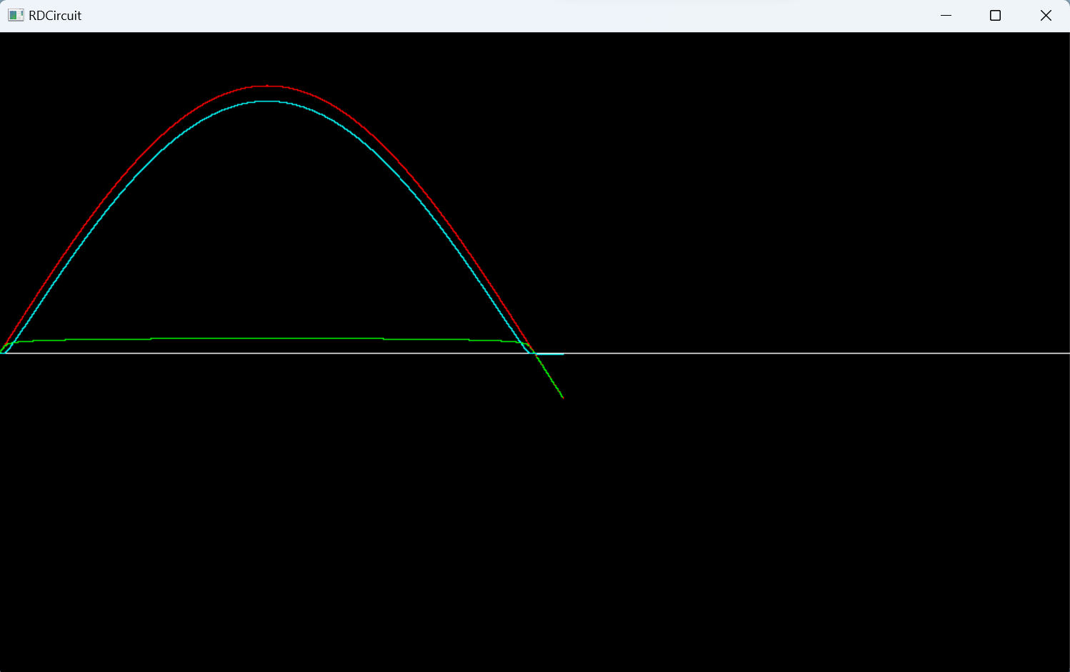
Sample Simulation - Resistor Diode Circuit
Files to simulate a resistor and diode in series with an AC voltage applied can be seen at:
Component.h, the component interface class,
Resistor.h, the resistor concrete component class,
Diode.h, the diode concrete component class,
RDMain.cpp, the simulation main function.
The circuit is shown below:
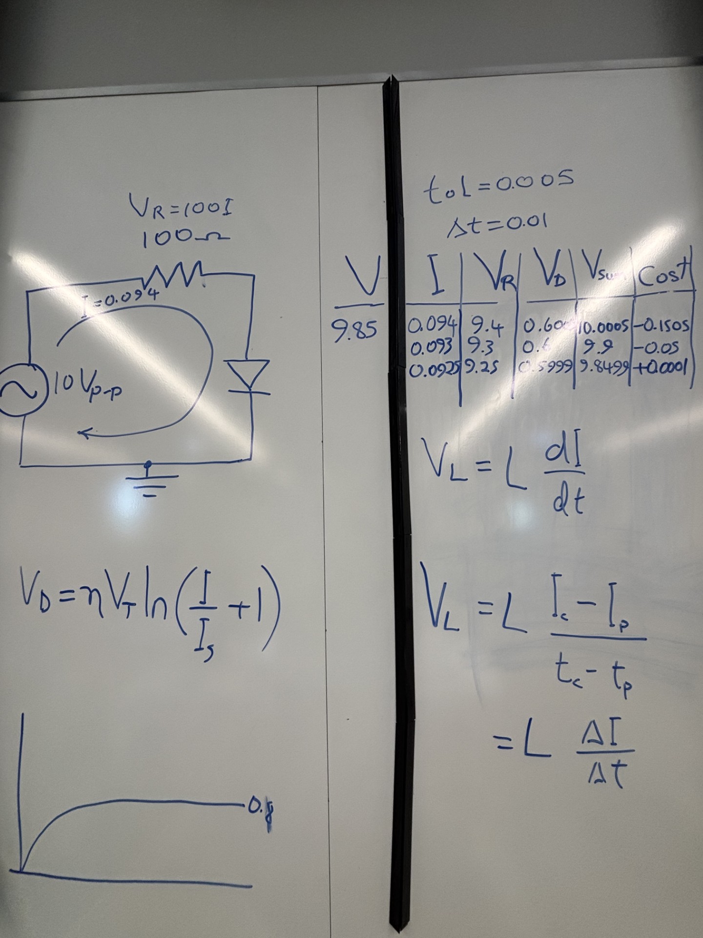
The same cost function has been used as in the assignment with one exception, the current cannot be less than the
saturation current of the diode. As you can see from the following image, the simulator works well when the
diode is forward biased, but breaks down when reverse biased: